#install.packages("ggplot2")If you are just getting started with R, I recommend following along with Kosuke Imai’s textbook Quantitative Social Science (https://press.princeton.edu/books/quantitative-social-science), especially if you are using R for political science or other social science applications. This post is tailored to those who are just starting out.
Installing R
First, make sure you have R installed, as well as RStudio. If you want to save your R code from any given session, you can create and save a .R script, or, an ‘R Markdown’ (.rmd) document to save the R code. R Markdown allows you to output your code, results such as tables and graphs, and additional writing as a PDF document, which can be convenient. R Markdown also lets you create different ‘chunks’ of code, with results displaying after each, which can help to keep things organized, compared to a simple .r script.
Typically, for installation, you will first need to go manually download an .exe file from a website. Then, finish any installation steps on your computer.
For Windows,
- Install R by going to https://cran.r-project.org/bin/windows/base/ (“CRAN”) and downloading the .exe file prominently linked on the page. You may need to select a “mirror” location – choose the one closest to you for a faster download.
- Install RStudio from https://posit.co/download/rstudio-desktop/. Again, you will need to right click and download the program file, then finish any installation steps by opening the program file on your device and following any remaining instructions. (R itself can also be downloaded from this link).
RStudio is essentially a program interface that makes working with R more user-friendly – you can see the working environment (files and other ‘objects’ you have loaded into or created in R), as well as your script, plots you might create, and a help window. It is possible to open and use R directly, but perhaps not advisable.1
How to update R and RStudio
Occasionally, you may need to move to a newer version of R and/or RStudio to keep everything running properly.
You can see which version of R you are running by opening the R program, or running “R.Version()” in RStudio.
On Mac: To update R, open the R program itself (which I have just told you to avoid), go to the “R” menu dropdown, and select ‘Check for updates’. Follow instructions to install.
On Windows: You can either manually un-install R, and start the installation process all over again from the installation instructions, or install the ‘installr’ package (with command: install.packages(“installr”), followed by command: “library(installr)” and then command: updateR().)
What is R?
R is an ‘object-oriented programming language’, which means you can create and name ‘objects’ of different kinds as you are working in a session. These might be: dataframes (a spreadsheet-style table of numbers or other data), lists, vectors (in computing, this means essentially an ordered list of numbers or other entries, such as text entries; any column of a spreadsheet is a vector) singular numbers, and more. You can also load data from files you have (often .csv for spreadsheet data, but other filetypes are possible), and save the output of your work as a file, but these require special commands and your work in any R session will not, by default, be saved to file.
What is a script? What is a package?
Each .r or .rmd script is a saved series of commands. These take whatever input you have defined, such as a dataset, and perform steps such as editing variables, calculating figures such as averages, and plotting graphs. In general, it is good practice to save your work as an R script so that you can recreate your steps at a later date. (This also may be required for publishing your work – increasingly, coding scripts and data files must be reported to journals so that your analysis can be checked and replicated).
Your script can be a cleaned up and edited version of commands you have run while in the R session. You can also run commands in the ‘console’, usually the bottom left window of RStudio, to obtain results without necessarily saving the commands you are running.
We will not deal with R packages in this post, but essentially, they are optional extensions of R that people have written to cover certain functions that might be difficult or require a large amount of “base R” (R itself, without packages) code to complete. Many regression models, plots, and other practical tasks (you can make R play a beeping sound when it has finished running something with the “beepr” package, or time how long something takes to run with the “tictoc” package, for example).
To install a package
For now, we will only install the very commonly used GGPlot package, which most scholars use to create plots in R, rather than R’s in-built plotting features, like “plot()” and “text()” (to add text labels to a plot). The official name of the package is “ggplot2”, in all-lowercase. In general, you must be extremely precise with capitalization and punctuation when running anything in R. It will not run if you are even one character off – at best, you will receive a useful red highlight or warning message that points you to where the problem character is.
Any package that is an official R package can be downloaded with:
Installing the package is a one-time event; you will not need to run this each time you open a session. (You may need to if you completely move to a new device or re-download R and RStudio, though).
Then, once per session, load the pack with:
library(ggplot2)Note that the installation command has quotation marks, but opening the library does not.
You can then use commands from the package.
(We will not use GGPlot yet; only base R for plotting in this post).
Common tasks
One more general point before starting is that you can think of R, or any coding language, as somewhat similar to a real language. Objects are like nouns; and commands like plot(), mean(), print(), c(), table() or length() are like verbs. These verb-like commands are called “functions”. They take an input object and return some type of output, such as printing a mean.
Create a dataframe
The word for spreadsheet or dataset in R is ‘dataframe’. This is a type of object that has columns (different variables), and rows of observations.
We can create a small one from scratch with the data.frame() function.
mydata = data.frame(Name = c("Alfred", "Alex", "George"),
                    Age = c(75, 34, 25),
                    Province = c("ON", "QC", "ON"))
We have just created a dataframe object called ‘mydata’. If you look at the top-right “Environment” window in RStudio, you should now be able to see the “mydata” object. If you click on it, it will show you the dataframe.
Alternatively, if we want to see the dataframe, we can type its name and it will print on-screen.
mydata Name Age Province
1 Alfred 75 ON
2 Alex 34 QC
3 George 25 ONWe now have a very simple dataset to work with.
Other than the data.frame() function, where we filled in relevant information as “arguments” within the brackets, we also used the c() function, which means ‘concatenate’, or, append several items together, in the order given.
Selecting variables and cells in a dataset
In the console, or in your script, R can work as a calculator on numeric objects.
To check what type of object something is, you can use the class() function, as shown below.
Note that a specific column of the dataframe can be selected with the $ character. (mydata$Name will select the Name column, for example).
You can use the hashtag sign to insert your own comments about the code. This is strongly recommended, as R syntax is not always highly intuitive, and so your plain-language comments will help later you remember what your code does and why you ran something in a particular way.
mydata$Name # Select this column; print to screen[1] "Alfred" "Alex" "George"Print to screen with print() or cat(), with the item or items you want printed in the brackets.
print(mydata$Age)[1] 75 34 25cat(mydata$Age)75 34 25Importantly, we can also stack and combine commands in R. R will run the inner command first, then the outer one. Brackets can also be used in math operations, to make R run commands in BEDMAS order.
cat(c(mydata$Name, mydata$Age))Alfred Alex George 75 34 25Select a particular cell in a dataframe with square brackets: Row number goes first (always), then a comma, then the column specification.
mydata[2, 1] # Row 2, column 1[1] "Alex"Select a whole column by number:
mydata[,1] # All rows; column 1[1] "Alfred" "Alex" "George"Just one dimension is needed if selecting from a list or vector:
mydata$Name[2] # 2nd item in Name column[1] "Alex"
Math in R
We can run math commands:
3+5[1] 83+5/8[1] 3.625(3+5)/8[1] 1To run any command in R, type it and either push Enter if you are working in the console, or Ctrl+Enter if working in a script. (On Windows). You can also highlight text and look for the ‘Run’ button in RStudio, but in general, learning the keyboard commands is more efficient.
Math functions, cont.
Mean, standard deviation, and median-finding functions are built into R. You may need to insert additional arguments to tell R what to do with any NA (blank) entries. Otherwise, your result may be NA if there is even one missing entry in the input.
mean(mydata$Age)[1] 44.66667We can round numbers (default: to whole numbers; this is changed to 2 decimal places with the “, 2” argument below):
round(mean(mydata$Age),2)[1] 44.67In general, spaces don’t matter as much as other characters and punctuation in R. One space or no spaces are typically equivalent to each other.
Counting
You can count the number of items with functions nrow() (for dataframes); or length() (for vectors or lists).
Summing values can be done with sum().
Detailed counts can also helpfully be seen with table().
nrow(mydata) # Number of rows[1] 3length(mydata$Age) # Also 3 rows[1] 3sum(mydata$Age) # Instead, sum values.[1] 134table(mydata$Province) # See counts under each existing value in the column.
ON QC
 2  1
Logical Statements (True or False Operators; “Booleans”)
A = 4 # Assign a value to an object with "=" or "<-".

B = 8

A > B # Is A greater than B?
[1] FALSEOperators include >, <, >= for ‘[a] is greater than or equal to [b]’; <= for ‘[a] is less than or equal to [b]’, == for ‘is [a] equal to [b]?’ (As opposed to “=” or “<-”, which set an assignment), and != for ‘is [a] NOT equal to [b]?’.
We also have “&” for ‘and’ – are A and B both true? and “|” for ‘or’.
A == B # Is A equal to B?[1] FALSEA != B # Is A NOT equal to B?[1] TRUE2*A == B # Is 2 times A equal to B?[1] TRUEMultiplication can be expressed with “*”, division with “/” (make sure to use brackets as needed); and exponents with “^” following a number. (Not exp(), which will give you the exponent on e (2.78…) needed to make e^(output number) equivalent to the number you put into the brackets).
# Consult R documentation for details and examples for any function:

#?sum

# or, equivalently,

#help(sum)
See problems with NAs here:
x_list = c(2, 3, 4, 5, 6, 8, NA, 10)

mean(x_list)
[1] NAmean(x_list, na.rm = T)[1] 5.428571
Strings; Factors; Text Entries
In computing, an entry that is a literal string of text is called a ‘string’. This could include: someone’s name, their gender spelled out as a word (and not as a number code), open-ended survey question responses, or closed-ended question responses (Strongly Agree; Disagree, etc; or province names, city names, and so on).
class(mydata$Name)[1] "character"For R, vectors consisting of text (strings) are now read in as ‘character’ type.
For some purposes, you may want to tell R to make them ‘factor’ type, which is less easily editable, and consists of a small number of discrete categories.
class(mydata$Province)[1] "character"mydata$Province = as.factor(mydata$Province) # Change type; reassignclass(mydata$Province)[1] "factor"You can also change numeric variables to factor type with as.factor(), for example for plotting or for regression models.
See also: as.character(), as.numeric() to change a variable into character type or numeric type; as.logical() to convert 1s and 0s into TRUEs and FALSEs, respectively.
Note that these functions all change the type of variable, if overwritten as shown above. To simply check the type, use class() or is.numeric(), is.factor(), is.logical(), which will return a TRUE or FALSE answer to the question.
Basic plotting
We will now make a new dataset with a time variable, year, and a second variable, voter turnout. Time is typically plotted on the x-axis, if it is one of the two variables in an x-y plot.
You can also plot any two variables together in an x-y format. Typically, the more stable or unchangeable one will go on the axis. If you have a causal theory in mind, where one variable (IV) affects another (DV), the IV will go on the x-axis.
# New dataframe

# Voter turnout data from Elections Canada,
# https://www.elections.ca/content.aspx?section=ele&dir=turn&document=index&lang=e

CanDF = data.frame(Year = c(1984, 1988, 1993, 1997,
                            2000, 2004, 2006, 2008,
                            2011, 2015, 2019, 2021),
                   Turnout = c(75.3, 75.3, 69.6, 67.0,
                               61.2, 60.9, 64.7, 58.8,
                               61.1, 68.3, 67.0, 62.6))
  # Make sure to close each set of brackets, and include commas in relevant places.

  # If you miss punctuation, you may get an 'unexpected symbol' error.
  # If you omit a needed bracket, you may get stuck in an unfinished command, with R
  # printing + symbols to the console.
We can plot in base R with the plot() command, with x = (variable) and y = (variable) arguments choosing the variable on each axis.
plot(x = CanDF$Year, y = CanDF$Turnout)

# Or, equivalently,

plot(CanDF$Year, CanDF$Turnout)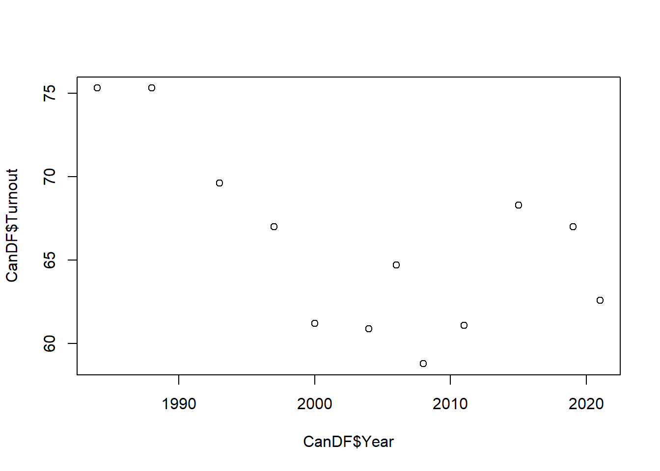
# Add a title with "main", change variable labels with "xlab" and "ylab".
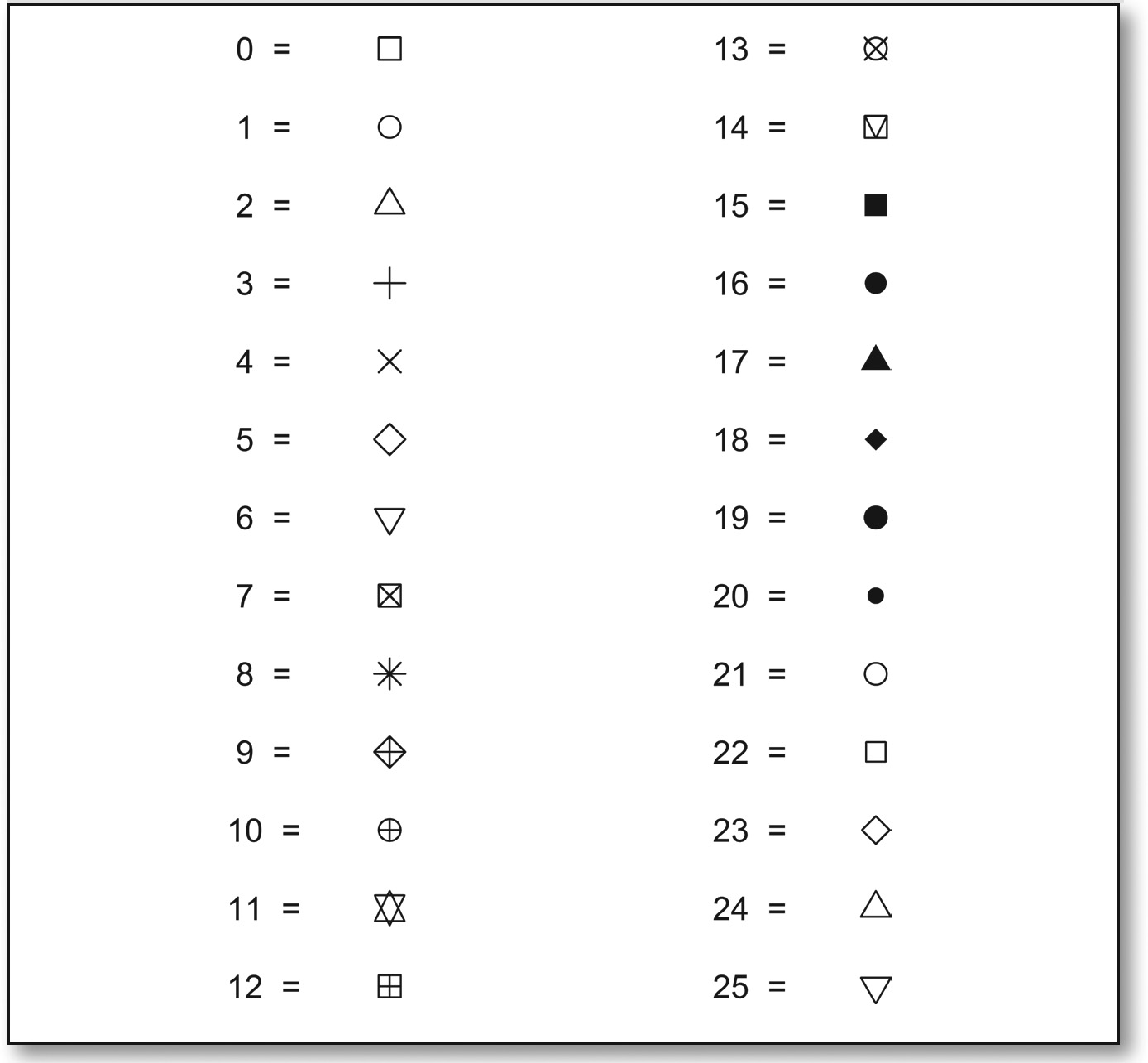
# Change point type with pch = 0, 1, 2, etc. (See options below; default = 1).
# Change font size ('character expansion') with cex = 0.8, 0.9, etc. (Default 1).
plot(CanDF$Year, CanDF$Turnout,
main = "Turnout in Canadian Elections 1984-2021",
xlab = "Year",
ylab = "Turnout Rate",
pch = 16)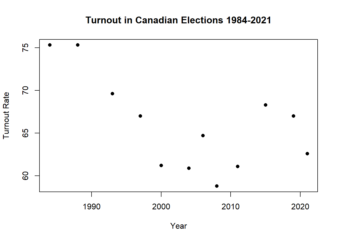
For the pch options, see image from Sage: https://www.google.com/url?sa=i&url=https%3A%2F%2Fmethods.sagepub.com%2Fbook%2Fa-survivors-guide-to-r%2Fi2014.xml&psig=AOvVaw24YVkuiZpkKTNOMKoQ2Fzz&ust=1692741996539000&source=images&cd=vfe&opi=89978449&ved=0CBIQjhxqFwoTCNDEk73h7oADFQAAAAAdAAAAABBQ.
You can also hide points on a base R plot with pch = ““.
Line graph
Draw a line and erase the points with “type = l”.
plot(CanDF$Year, CanDF$Turnout,
     main = "Turnout in Canadian Elections 1984-2021",
     xlab = "Year",
     ylab = "Turnout Rate",
     type = "l",
     pch = 6)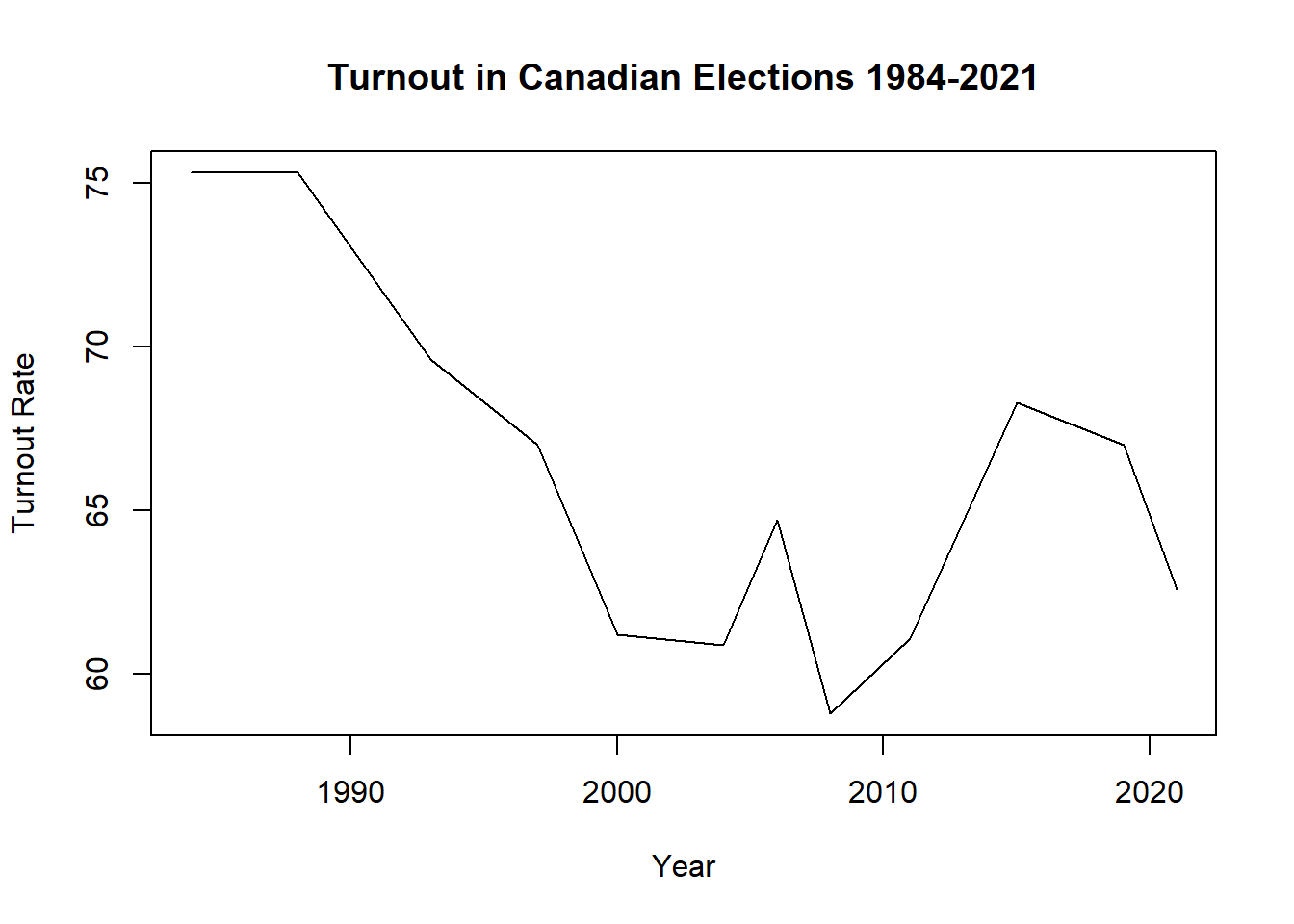
Or, you can layer commands, and keep the datapoints visible if you want:
plot(CanDF$Year, CanDF$Turnout,
     main = "Turnout in Canadian Elections 1984-2021",
     xlab = "Year",
     ylab = "Turnout Rate",
     pch = 22)
lines(CanDF$Year, CanDF$Turnout)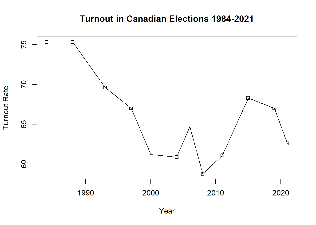
Change the x and y axes with xlim and ylim, specifying the two extreme points.
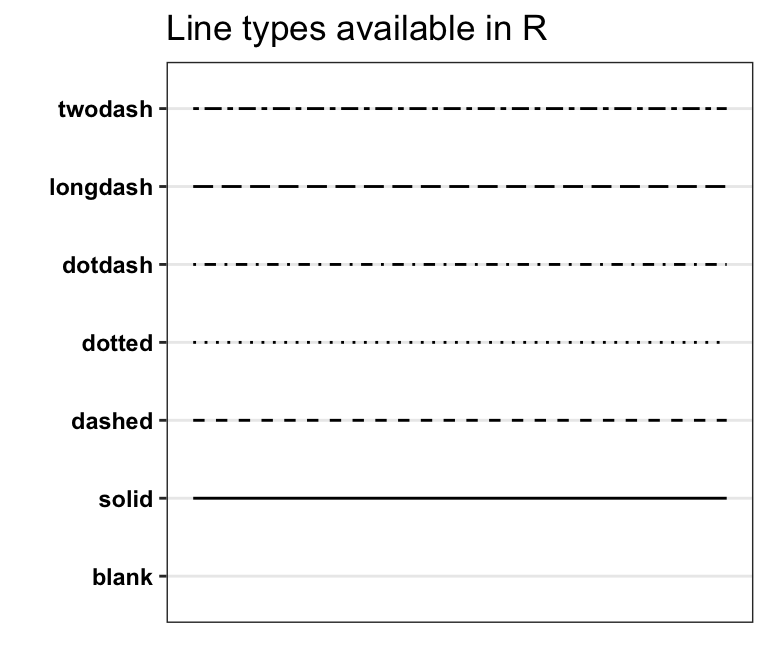
Change line weight (thickness) with lwd = ; line dashing with lty = ; colour of points or lines with col = “black”, “red”, “#EEAA88”, etc.
Line type options, image from Data Novia: https://www.google.com/url?sa=i&url=https%3A%2F%2Fwww.datanovia.com%2Fen%2Fblog%2Fline-types-in-r-the-ultimate-guide-for-r-base-plot-and-ggplot%2F&psig=AOvVaw1s4DY9T3HyjKt4eA8KLuLB&ust=1692742603628000&source=images&cd=vfe&opi=89978449&ved=0CBIQjhxqFwoTCMDI097j7oADFQAAAAAdAAAAABAE.
plot(CanDF$Year, CanDF$Turnout,
     main = "Turnout in Canadian Elections 1984-2021",
     ylim = c(40, 100),
     xlab = "Year",
     ylab = "Turnout Rate",
     pch = 18, col = "black")
lines(CanDF$Year, CanDF$Turnout, lwd = 2, lty = "longdash",
      col = "#88AAEE")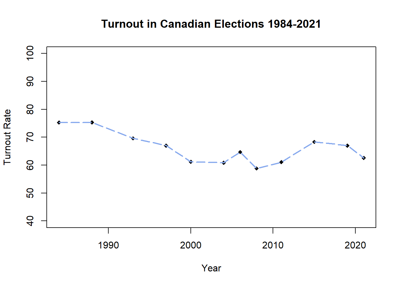
Customize the x-axis values by erasing the x-axis from the main plot and re-adding a custom one with axis():
plot(CanDF$Year, CanDF$Turnout,
     main = "Turnout in Canadian Elections 1984-2021",
     ylim = c(40, 100),
     xaxt = "n", # Erase x axis markings here
     xlab = "Year",
     ylab = "Turnout Rate",
     pch = 18, col = "black")
lines(CanDF$Year, CanDF$Turnout, lwd = 2, lty = "longdash",
      col = "#88AAEE")
axis(side=1, at = seq(1984, 2022, by = 2)) # Seq() prints a series of numbers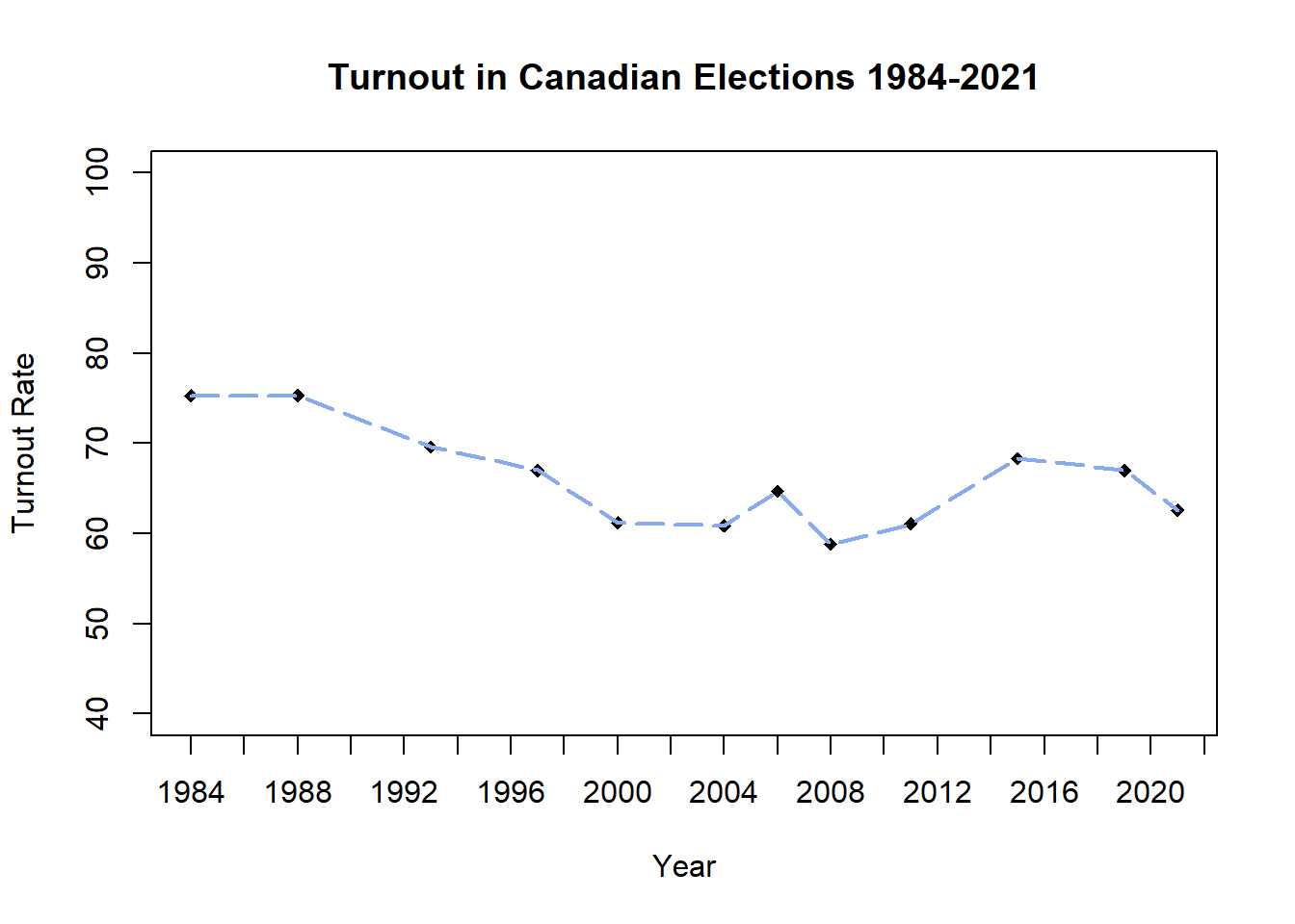
Colours, cont.
To view all the colours you can call by name, check colours() or colors(). (Both British/Canadian and American spellings will typically work for referring to colour commands in R, and in GGplot.)
Preview the first few elements of something (a list, a dataframe) with head(). Tail (“tail()”) will print the last few.
#colours() # Print all 657

head(colours()) # Show first few entries (Default is 6)
[1] "white" "aliceblue" "antiquewhite" "antiquewhite1"
[5] "antiquewhite2" "antiquewhite3"head(colours(), 30) # Print first 30 [1] "white" "aliceblue" "antiquewhite" "antiquewhite1"
[5] "antiquewhite2" "antiquewhite3" "antiquewhite4" "aquamarine"
[9] "aquamarine1" "aquamarine2" "aquamarine3" "aquamarine4"
[13] "azure" "azure1" "azure2" "azure3"
[17] "azure4" "beige" "bisque" "bisque1"
[21] "bisque2" "bisque3" "bisque4" "black"
[25] "blanchedalmond" "blue" "blue1" "blue2"
[29] "blue3" "blue4" You can also work in RGB format (#000000 = black, #FFFFFF = white, #FF0000 = red, etc.), with an optional two digits at the end to set transparency level (‘alpha’; 00 = lowest opacity; FF = highest opacity).
plot(CanDF$Year, CanDF$Turnout,
     main = "Turnout in Canadian Elections 1984-2021",
     ylim = c(40, 100),
     xaxt = "n", # Erase x axis markings here
     xlab = "Year",
     ylab = "Turnout Rate",
     pch = 18, col = "#FF002266")
lines(CanDF$Year, CanDF$Turnout, lwd = 2, lty = "longdash",
      col = "#88AAEE44")
axis(side=1, at = seq(1984, 2022, by = 2))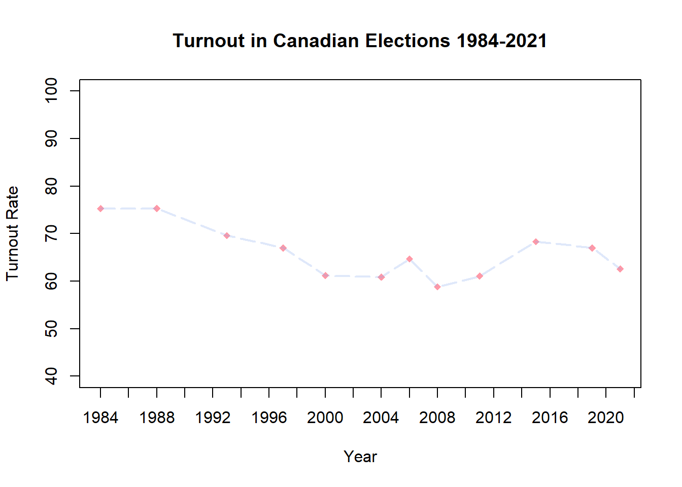
Have fun getting started!
Footnotes
You may need to open the R program directly to update R itself, or to update certain packages for developers.↩︎